Section 1.1: What is a Confidence Interval?

To illustrate confidence intervals, consider a shopping mall aiming to estimate the number of customers it receives on weekdays from 9 am to 12 pm. They can sample data from around 100 weekdays to compute the average. Suppose the calculated average is 42 customers, with a population standard deviation of 15.

According to the Central Limit Theorem (CLT), the sample mean should approximate the true population mean. However, this sample mean may differ if larger samples, say 1000 or 10,000, are taken. How do we infer the true population mean from this sample mean?

By utilizing the sample size, sample mean, and population standard deviation, we can establish a range that is expected to contain the true population mean, known as the confidence interval.

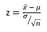
For our example, with n ≥ 30, the sample mean can be presumed to be normally distributed. The standard deviation formula is as follows:

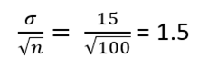
This standard deviation indicates that 95% of sample means will lie within two standard deviations of the true population mean, adhering to the 68–95–99 rule. Thus, 95% of the time, the population mean will be within 1.5 standard deviations of the sample mean.

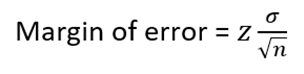
Here is the general formula for calculating a confidence interval:

The estimate derives from the sample mean, while the margin of error indicates how far the population mean might deviate from the sample mean.

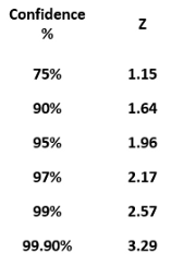
The critical z-value remains constant across various confidence levels. Below is a chart depicting commonly used confidence levels:

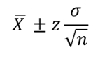
The comprehensive formula for the confidence interval is thus:

Continuing with our shopping mall example, the upper limit of the 95% confidence interval is calculated as follows:

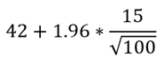
This results in an upper limit of 51.3, while the lower limit is:

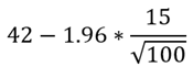
Thus, the confidence interval ranges from 32.7 to 51.3, indicating a 95% confidence that the true average number of customers in the mall during weekdays from 9 am to 12 pm falls between these values.

Now that we have a foundational understanding of confidence intervals, we will explore how to compute them using R in various examples.

Section 1.2: Hypothesis Testing

Hypothesis testing involves assessing evidence for a specific claim regarding a population. To exemplify this, imagine I claim I can swim ten consecutive laps in a 40-foot pool. If I can only manage four laps before tiring, would anyone still believe my assertion?

In hypothesis testing, we gather evidence regarding a particular claim. If a hypothesis about a population proves to be exceedingly rare compared to the true value, we reject that claim. Probabilities help assess the rarity of the claim, so let’s examine an example to clarify the process.

Example 1:

A teacher introduces a new reading method and wants to determine its effectiveness on student scores. Unable to assess every student in the world, the teacher samples 60 students, observing an average score increase to 6.5 with a population standard deviation of 11. We will evaluate if this new method has genuinely improved scores at a 95% confidence level.

We will follow a structured five-step process for hypothesis testing. First, we’ll begin with the manual calculations, followed by an expedited R function.

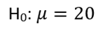
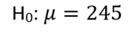
Step 1: State the hypotheses. The null hypothesis posits no change in scores due to the new method, expressed as:

Should we find insufficient evidence to support the null hypothesis, we will then accept the alternative hypothesis, indicating that the mean score has improved.

Step 2: Select the appropriate test statistic. Given a sample size of 60 with a known population standard deviation, a z-statistic is suitable.

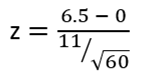
Step 3: Calculate the z-statistic:

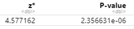
The calculated z-statistic is 4.58. We can derive the p-value from this statistic.

From the above representation, the test statistic is depicted as a point, while the p-value represents the area beneath the curve. This p-value indicates the likelihood of observing the calculated test statistic or one more extreme, assuming the null hypothesis holds true.

Using R, the p-value can be easily computed from the z-statistic, as illustrated in the following article:

The second video provides insights into confidence intervals in R, which can further enhance your understanding of this topic:

Step 4: Establish the decision rule. With a confidence level of 95%, the significance level (alpha) is set at 5% or 0.05. We will reject the null hypothesis if the alpha value is less than the p-value.

Step 5: Draw conclusions. Given the p-value of 2.325e-06, which is significantly smaller than the alpha value, we reject the null hypothesis. This indicates that the new reading method has effectively improved student scores.

Using R simplifies these calculations significantly. With the 'asbio' package, finding the z-statistic and p-value is straightforward. The function one.sample.z can be employed for this purpose as shown below:

Example 2:

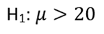
In another scenario, a scientist measures ten great white sharks to test if their average length exceeds 20 feet. The calculated sample mean is 22.27 feet, with a sample standard deviation of 3.19. We will use the same five-step hypothesis testing approach as before.

Step 1: Formulate the hypothesis and alpha level. The null hypothesis posits that the average length of great white sharks is 20 feet.

If sufficient evidence is found to reject this null hypothesis, we will accept the alternative hypothesis.

Step 2: Select the appropriate test statistic. Given a sample size of 10 and unknown population standard deviation, a t-statistic is the appropriate choice.

Step 3: Calculate the t-statistic. Although the formula is available, R can quickly compute the t-statistic and p-value in one line:

x = c(21.8, 22.7, 17.3, 26.1, 26.4, 21.1, 19.8, 24.1, 18.3, 25.1)

t.test(x, mu = 20, alternative = "greater")

The output will provide the t-statistic and p-value.

Step 4: Set the decision rule. If the p-value is less than or equal to the alpha level, we reject the null hypothesis.

Step 5: Draw the conclusion. Since the p-value is 0.025, which is less than the significance level of 0.05, we have enough evidence to reject the null hypothesis. Therefore, the average length of great white sharks is likely greater than 20 feet.

The next few examples will focus on comparing two means, utilizing the heart disease dataset from Kaggle.

Example 3:

We will assess whether the cholesterol levels of the male population are lower than those of the female population at a significance level of 0.05.

Step 1: Establish the hypothesis and alpha level. The null hypothesis posits that the mean cholesterol levels of males and females are equal.

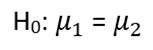
The alternative hypothesis states that the male population's mean cholesterol is less than that of the female population.

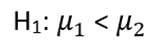
Step 2: Choose the appropriate test statistic. A t-statistic is commonly employed for comparing two means:

Step 3: Compute the t-statistic and p-value. First, load the heart dataset into R:

h = read.csv('Heart.csv')

Using the t.test function, we can evaluate the cholesterol levels:

t.test(h$Chol[h$Sex=='1'], h$Chol[h$Sex=='0'], alternative = 'less', conf.level = 0.95)

The output will yield the t-statistic and p-value.

Step 4: State the decision rule. If the p-value is less than alpha, reject the null hypothesis.

Step 5: Draw the conclusion. If the p-value indicates statistical significance, it suggests that male cholesterol levels are indeed lower than those of females.

Moving forward, we will explore how to perform a two-sided z-test and calculate a confidence interval utilizing the heart dataset.

Example 4:

We will verify whether the population mean cholesterol level is 245 and construct a confidence interval around the mean cholesterol level at a significance level of 0.05.

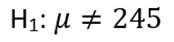
Solution: The null hypothesis states:

The alternative hypothesis indicates that the mean cholesterol level differs from 245.

Using the z-test, we can obtain the z-statistic, p-value, and confidence interval in one simple command:

z.test(h$Chol, NULL, alternative = "two.sided", mu = 245, sigma.x = sd(h$Chol), sigma.y = NULL, conf.level = 0.95)

The output will reveal if the null hypothesis can be rejected.

We will also touch upon tests for proportions in subsequent examples.