Theory

Integrating a function over a defined interval [a, b] allows us to calculate the area beneath the curve between these two points. The definite integral can be represented mathematically as shown in Equation 1.

While there are various methods for deriving the analytical solution for a definite antiderivative, some functions pose challenges that prevent expressing their antiderivatives using standard functions.

Techniques

To estimate the area between the x-axis and a curve f(x), one can utilize a Riemann sum, which involves adding up numerous smaller sections of the total area. Below are Python implementations for three prevalent numerical integration methods:

1. Trapezoidal Rule
2. Midpoint Rule
3. Simpson’s Rule

Each of these integration techniques requires calculating the continuous function f(x) at n+1 evenly spaced intervals within [a, b]. The step size between points is defined in Equation 2.

The most efficient numerical integration techniques yield a sufficiently accurate integral approximation while minimizing the number of f(x) evaluations.

Trapezoidal Rule

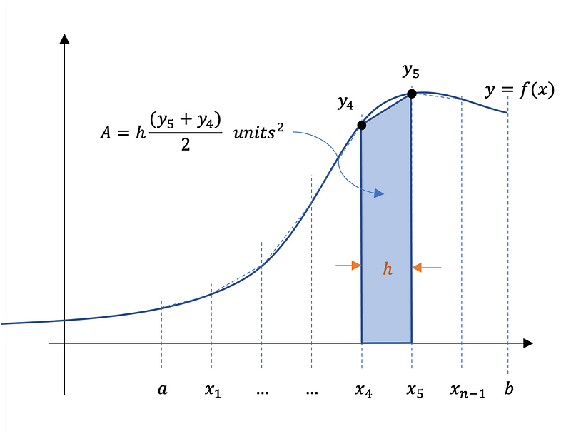
The area of a trapezoid, which is a four-sided shape with two parallel sides, can be determined using Equation 3.

Figure 1 illustrates how the area is divided using n trapezoids, where the sum of the individual trapezoidal areas approximates the total area.

Equation 4 outlines the trapezoidal rule for numerical integration, and Gist 1 provides a Python implementation detailing each step.

Midpoint Rule

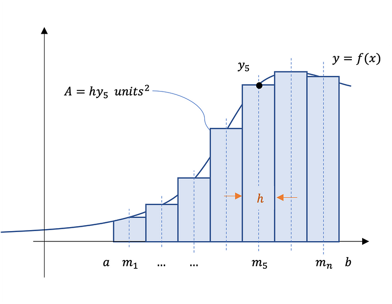
The midpoint rule estimates a definite integral by employing a Riemann sum of rectangles, where the rectangle heights correspond to f(x) evaluated at the midpoints of the n subintervals. Figure 2 depicts the subintervals, midpoints, and the rectangles.

Equation 5 determines the midpoints of the subintervals.

Using a as the beginning of the interval, h as the step size, and n as the number of subintervals, Equation 6 defines the midpoint rule.

The area approximation is computed by summing the areas of the rectangles, which represent the area between the function f(x) and the x-axis across the specified interval. Gist 2 presents the Python code for the midpoint rule.

Simpson’s Rule

Simpson’s rule enhances the approximation of a definite integral by employing quadratic functions, generally providing more accurate results than the previously discussed methods. Equation 7 illustrates Simpson’s rule for numerical integration.

To utilize Simpson’s rule, at least three sampling points are required, necessitating an odd total number of sampling points, meaning that the number of subintervals n must be even. Gist 3 provides the Python code for implementing Simpson’s rule.

Error Estimations

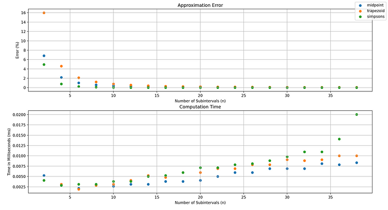
Two critical metrics for evaluating the performance of these techniques are the approximation error and the computation time. Let f(x) be defined as shown in Equation 8.

Equation 9 presents the analytical integral used for demonstration purposes. Numerical integration is typically necessary when an analytical solution is not available.

For this analysis, the chosen interval is [2, 10], with the expected value calculated to 17 significant figures being 1.6094379124341005. The estimation error quantifies the difference between the calculated value and the expected value, as defined in Equation 10.

Here, the measured value refers to the approximation derived from numerical integration. Figure 3 presents a plot of the errors and computation times for the trapezoidal, midpoint, and Simpson’s rule applied to Equation 8 to approximate Equation 9 with increasing subintervals.

Conclusion

The results indicate that as the number of subintervals increases, the computation time also rises, while the error diminishes. The provided Python implementations do not prioritize performance optimization, so there is potential for improvements. Among the techniques discussed, Simpson’s rule tends to yield the most precise approximations, albeit at a higher computational cost.

This guide has demonstrated how to perform numerical integration in Python using the trapezoidal, midpoint, and Simpson’s rules.

This video titled "Integration in PYTHON (Symbolic AND Numeric)" provides an overview of various integration techniques in Python, including symbolic and numerical integration methods.

The video titled "Numerical Integrals in Python" dives deeper into the different numerical methods for integration, offering practical examples and explanations.